Step-by-Step Tutorial on Reinforcement Learning

Step 1: Understand the Core Concepts of Reinforcement Learning

Reinforcement learning revolves around an agent interacting with an environment to learn a policy that maximizes a reward. Here’s a breakdown of the key components:

• Agent: The decision-maker (e.g., a robot, a game player).
• Environment: The world the agent interacts with (e.g., a game, a simulation).
• State (s): A representation of the environment at a given time (e.g., the position of a player in a game).
• Action (a): The choices the agent can make (e.g., move left, jump).
• Reward (r): A scalar feedback signal from the environment after an action (e.g., +1 for a good move, -1 for a bad one).
• Policy (π): A strategy that maps states to actions (e.g., “if in state s, take action a”).
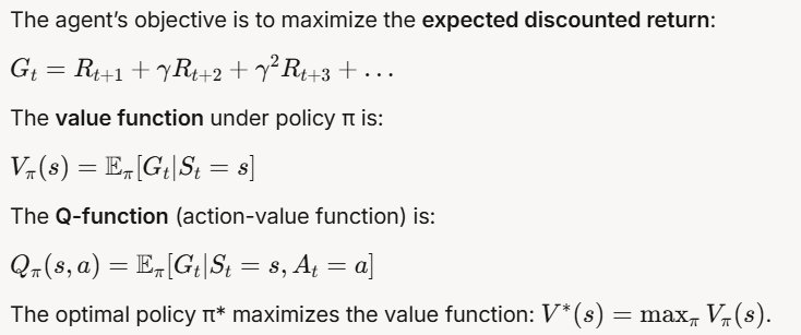
• Value Function (V): Estimates the expected cumulative reward starting from a state, following a policy.
• Q-Function (Q): Estimates the expected cumulative reward for taking a specific action in a state and following a policy thereafter.

The goal of RL is to find an optimal policy (π*) that maximizes the expected cumulative reward over time, often discounted by a factor γ (gamma) to prioritize immediate rewards over distant ones.

---

Step 2: Grasp the Mathematical Framework

Reinforcement learning is often modeled as a Markov Decision Process (MDP), defined by the tuple (S, A, P, R, γ):

• S: Set of states.
• A: Set of actions.
• P(s’|s, a): Transition probability of moving to state s’ from state s after taking action a.
• R(s, a, s’): Reward function for transitioning from s to s’ via action a.
• γ: Discount factor (0 ≤ γ < 1), balancing immediate vs. future rewards.

The agent’s objective is to maximize the expected discounted return:

---

Step 3: Choose an RL Algorithm

For this tutorial, we’ll focus on Q-Learning, a simple yet powerful model-free RL algorithm. Q-Learning is an off-policy algorithm, meaning it learns the optimal policy even if the agent doesn’t follow it during training. It updates the Q-values using the Bellman equation:

Where:

• α: Learning rate (how much to update Q-values).
• r: Immediate reward.
• γ: Discount factor.
• s’: Next state.
• a’: Next action.

Q-Learning uses an ε-greedy policy to balance exploration (trying new actions) and exploitation (choosing the best-known action):

• With probability ε, pick a random action.
• With probability (1-ε), pick the action with the highest Q-value.

---

Step 4: Set Up the Environment

We’ll use the OpenAI Gym library (now part of Gymnasium) to create a simple environment for our RL agent. The “FrozenLake-v1” environment is a good starting point. It’s a grid world where the agent must navigate from a start to a goal while avoiding holes.

Install Dependencies

First, install Gymnasium if you haven’t already:

pip install gymnasium

Create the Environment

Here’s the setup in Python:

import gymnasium as gym
import numpy as np

# Create the FrozenLake environment
env = gym.make("FrozenLake-v1", is_slippery=False)
env.reset()

# Get the state and action space sizes
n_states = env.observation_space.n  # 16 states in a 4x4 grid
n_actions = env.action_space.n     # 4 actions (left, down, right, up)

In FrozenLake:

• States: 16 positions on a 4×4 grid.
• Actions: 4 directions (0: left, 1: down, 2: right, 3: up).
• Rewards: +1 for reaching the goal, 0 otherwise.
• The agent starts at (0,0) and aims to reach the goal (3,3).

---

Step 5: Initialize the Q-Table

The Q-table stores the Q-values for each state-action pair. Initialize it with zeros:

# Initialize Q-table with zeros
Q = np.zeros((n_states, n_actions))

# Set hyperparameters
alpha = 0.1    # Learning rate
gamma = 0.99   # Discount factor
epsilon = 0.1  # Exploration rate
n_episodes = 1000  # Number of training episodes
max_steps = 100    # Max steps per episode

---

Step 6: Implement the Q-Learning Algorithm

Now, let’s write the training loop for Q-Learning. The agent will:

1. Choose an action using the ε-greedy policy.
2. Take the action, observe the reward and next state.
3. Update the Q-table using the Bellman equation.
4. Repeat until the episode ends (goal reached or max steps exceeded).

# Training loop
for episode in range(n_episodes):
    state, _ = env.reset()  # Reset environment, get initial state
    done = False
    step = 0

    while not done and step < max_steps:
        # Choose action (ε-greedy)
        if np.random.uniform(0, 1) < epsilon:
            action = env.action_space.sample()  # Explore: random action
        else:
            action = np.argmax(Q[state, :])  # Exploit: best action

        # Take action, observe reward and next state
        next_state, reward, done, truncated, _ = env.step(action)

        # Update Q-table
        Q[state, action] = Q[state, action] + alpha * (
            reward + gamma * np.max(Q[next_state, :]) - Q[state, action]
        )

        # Move to the next state
        state = next_state
        step += 1

    # Optional: Decay epsilon to reduce exploration over time
    epsilon = max(0.01, epsilon * 0.995)

print("Training completed!")

---

Step 7: Test the Learned Policy

After training, test the agent by following the learned policy (always choosing the action with the highest Q-value):

# Test the agent
state, _ = env.reset()
done = False
total_reward = 0

while not done:
    action = np.argmax(Q[state, :])  # Choose the best action
    next_state, reward, done, truncated, _ = env.step(action)
    total_reward += reward
    state = next_state
    env.render()  # Visualize the agent's moves (if render mode is enabled)

print(f"Total reward: {total_reward}")
env.close()

In FrozenLake, a total reward of 1.0 means the agent successfully reached the goal.

---

Step 8: Analyze and Improve

• Results: After 1000 episodes, the agent should learn a policy that reliably reaches the goal. If not, try adjusting hyperparameters (e.g., increase n_episodes, tweak alpha or gamma).
• Exploration vs. Exploitation: If the agent gets stuck, increase epsilon to encourage more exploration. If it takes too long to converge, reduce epsilon or decay it faster.
• Environment Complexity: FrozenLake is simple. For more complex environments (e.g., CartPole-v1), you might need advanced algorithms like Deep Q-Learning (DQN), which uses neural networks to approximate the Q-function.

---

Step 9: Explore Advanced RL Techniques

Once you’re comfortable with Q-Learning, consider these next steps:

• Deep Q-Learning (DQN): Uses a neural network to handle large state spaces (e.g., for Atari games).
• Policy Gradient Methods: Directly optimize the policy (e.g., REINFORCE, PPO).
• Actor-Critic Methods: Combine value-based and policy-based methods for better stability (e.g., A3C, SAC).
• Multi-Agent RL: Train multiple agents to cooperate or compete (e.g., in games like soccer).

---

Step 10: Apply RL to Real-World Problems

Reinforcement learning has applications in:

• Robotics: Teaching robots to walk or grasp objects.
• Gaming: Training AI to play games like chess or Go.
• Autonomous Driving: Optimizing navigation and decision-making.
• Finance: Portfolio management and trading strategies.

Start with a small project, like training an RL agent to play a simple game, and gradually tackle more complex challenges.

---

This tutorial provides a foundational understanding of reinforcement learning through Q-Learning. By experimenting with the code and exploring advanced techniques, you’ll be well on your way to mastering RL and applying it to real-world problems. Happy learning!